travelling wave solution fisher's equation

• Open access
• Published: 18 December 2014

The general traveling wave solutions of the Fisher type equations and some related problems

• Wenjun Yuan 1 , 2 ,
• Bing Xiao 3 ,
• Yonghong Wu 4 &
• Jianming Qi 5  

Journal of Inequalities and Applications volume  2014 , Article number:  500 ( 2014 ) Cite this article

1565 Accesses

9 Citations

Metrics details

In this article, we introduce two recent results with respect to the integrality and exact solutions of the Fisher type equations and their applications. We obtain the sufficient and necessary conditions of integrable and general meromorphic solutions of these equations by the complex method. Our results are of the corresponding improvements obtained by many authors. All traveling wave exact solutions of many nonlinear partial differential equations are obtained by making use of our results. Our results show that the complex method provides a powerful mathematical tool for solving a great number of nonlinear partial differential equations in mathematical physics. We will propose four analogue problems and expect that the answer is positive, at last.

MSC: 30D35, 34A05.

1 Introduction

Nonlinear partial differential equations (NLPDEs) are widely used as models to describe many important dynamical systems in various fields of science, particularly in fluid mechanics, solid state physics, plasma physics and nonlinear optics. Exact solutions of NLPDEs of mathematical physics have attracted significant interest in the literature. Over the last years, much work has been done on the construction of exact solitary wave solutions and periodic wave solutions of nonlinear physical equations. Many methods have been developed by mathematicians and physicists to find special solutions of NLPDEs, such as the inverse scattering method [ 1 ], the Darboux transformation method [ 2 ], the Hirota bilinear method [ 3 ], the Lie group method [ 4 ], the bifurcation method of dynamic systems [ 5 – 7 ], the sine-cosine method [ 8 ], the tanh-function method [ 9 , 10 ], the Fan-expansion method [ 11 ], and the homogenous balance method [ 12 ]. Practically, there is no unified technique that can be employed to handle all types of nonlinear differential equations. Recently, Kudryashov et al. [ 13 – 16 ] found exact meromorphic solutions for some nonlinear ordinary differential equations by using Laurent series and gave some basic results. Following their work, the complex method was introduced by Yuan et al. [ 17 – 19 ]. In this article, we survey two recent results with respect to the integrality and exact solutions of the Fisher type equations and their applications. We obtain the sufficient and necessary conditions of integrable and general meromorphic solutions of these equations by the complex method. Our results are of the corresponding improvements obtained by many authors. All traveling wave exact solutions of many nonlinear partial differential equations are obtained by making use of our results. Our results show that the complex method provides a powerful mathematical tool for solving a great number of nonlinear partial differential equations in mathematical physics. We will propose four analogue problems and expect that the answer is positive, at last.

2 Fisher type equations with degree two

In 2013, Yuan et al. [ 17 ] derived all traveling wave exact solutions by using the complex method for a type of ordinary differential equations (ODEs)

where A , B , C and D are arbitrary constants.

In order to state these results, we need some concepts and notations.

A meromorphic function w ( z ) means that w ( z ) is holomorphic in the complex plane ℂ except for poles. α , b , c , c i and c i j are constants which may be different from each other in different place. We say that a meromorphic function f belongs to the class W if f is an elliptic function, or a rational function of e α z , α ∈ C , or a rational function of z .

Theorem 2.1 Suppose that A C ≠ 0 , then all meromorphic solutions w of Eq . (1) belong to the class W . Furthermore , Eq . (1) has the following three forms of solutions :

The elliptic general solutions

Here , 4 D C = − 12 A 2 g 2 + B 2 , F 2 = 4 E 3 − g 2 E − g 3 , g 3 and E are arbitrary .

The simply periodic solutions

where 4 D C = − A 2 α 4 + B 2 , z 0 ∈ C .

The rational function solutions

where 4 C D = B 2 , z 0 ∈ C .

Equation ( 1 ) is an important auxiliary equation, because many nonlinear evolution equations can be converted to Eq. ( 1 ) using the traveling wave reduction. For instance, the classical KdV equation, the Boussinesq equation, the ( 3 + 1 ) -dimensional Jimbo-Miwa equation and the Benjamin-Bona-Mahony equation can be converted to Eq. ( 1 ) [ 17 ].

In 2013, Yuan et al. [ 20 ] employed the complex method to obtain first all meromorphic solutions of the equation

where A , B , C , D , E are arbitrary constants.

Theorem 2.2 Suppose that A D ≠ 0 , then Eq . (2) is integrable if and only if B = 0 , ± 5 6 − 2 A D C 2 4 D 2 − E D , ± 5 i 6 − 2 A D C 2 4 D 2 − E D . Furthermore , the general solutions of Eq . (1) are of the following form :

If B = 0 , then we have the elliptic general solutions of Eq . (2)

Here , 12 A 2 g 2 = C 2 , M 2 = 4 N 3 − g 2 N − g 3 , g 3 and N are arbitrary .

In particular , which degenerates to the simply periodic solutions

where A 2 α 4 = C 2 , z 0 ∈ C .

And the rational function solutions

where C 2 = 4 D E , z 0 ∈ C .

If B = ± 5 6 − 2 A D C 2 4 D 2 − E D , then the general solutions of Eq . (2)

where C 2 4 D 2 = − C 2 D , both s 0 and g 3 are arbitrary constants .

In particular , which degenerates to the one parameter family of solutions

where C 2 4 D 2 = − C 2 D , z 0 ∈ C .

If B = ± 5 i 6 − 2 A D C 2 4 D 2 − E D , then the general solutions of Eq . (2)

where C 2 4 D 2 = − C 2 D , and both s 0 and g 3 are arbitrary constants .

The Fisher equation with degree two

Consider the Fisher equation

which is a nonlinear diffusion equation as a model for the propagation of a mutant gene with an advantageous selection intensity s . It was suggested by Fisher as a deterministic version of the stochastic model for the spatial spread of a favored gene in a population in 1936.

Set t ′ = s t and x ′ = ( s v ) 1 2 x and drop the primes, then the above equation becomes

By substituting

into Eq. (Fisher) and integrating it, we obtain

It is converted to Eq. ( 2 ), where

Three nonlinear pseudoparabolic physical models

The one-dimensional Oskolkov equation, the Benjamin-Bona-Mahony-Peregrine-Burgers equation and the Oskolkov-Benjamin-Bona-Mahony-Burgers equation are the special cases of our Eq. ( 2 ).

The one-dimensional Oskolkov equation has the form

where λ ≠ 0 , α ∈ R .

Substituting

into Eq. (Oskolkov) and integrating the equation, we have

The Benjamin-Bona-Mahony-Peregrine-Burgers equation is of the form

where α is a positive constant, θ and β are nonzero real numbers.

into Eq. (BBMPB), we get

The Oskolkov-Benjamin-Bona-Mahony-Burgers equation is of the form

where α is a positive constant, θ is a nonzero real number.

into Eq. (OBBMB), we deduce

The KdV-Burgers equation

The KdV-Burgers equation is of the form

where α is a constant.

Substituting the traveling wave transformation

into Eq. (KdV-B) and integrating it yields the auxiliary ordinary differential equation

where E is an integral constant. It is converted to Eq. ( 2 ), where

3 Fisher type equations with degree three

In 2012, Yuan et al. [ 21 ] employed the complex method to find all meromorphic solutions of the auxiliary ordinary differential equations

Theorem 3.1 [ 21 ]

Suppose that A C ≠ 0 , then all meromorphic solutions w of Eq . (3) belong to the class W . Furthermore , Eq . (3) has the following three forms of solutions :

The elliptic function solutions

Here , g 3 = 0 , d 2 = 4 c 3 − g 2 c , g 2 and c are arbitrary .

where z 0 ∈ C , B = A α 2 ( 1 2 + 3 2 sinh 2 α 2 z 1 ) , D = − A 2 C tanh α 2 z 1 sinh 2 α 2 z 1 , z 1 ≠ 0 in the former formula , or B = A α 2 2 , D = 0 .

where z 0 ∈ C . B = 0 , D = 0 in the former case , or given z 1 ≠ 0 , B = 6 A z 1 2 , D = ∓ 2 C ( − 2 A C z 1 2 ) 3 / 2 .

In 2013, Yuan et al. [ 22 ] considered the following equation:

where A , B , C and D are arbitrary constants. They obtained the following result and gave its two applications.

Theorem 3.2 Suppose that A ≠ 0 , then all meromorphic solutions w of Eq . (4) belong to the class W . Furthermore , Eq . (4) has the following three forms of solutions :

All elliptic function solutions

where A ( C 2 − 9 B ) = 12 C − A 2 , 27 D = C 3 , g 3 = 0 , F 2 = 4 E 3 − g 2 E , g 2 and E are arbitrary constants .

All simply periodic solutions

where z 0 ∈ C . A ( 2 C 2 + 9 A α 2 − 18 B ) = 24 C − A 2 , 27 D − C 3 = 27 α 2 − A 2 in the former case , or z 1 ≠ 0 , 8 C − A 2 + 6 A B = 3 A 2 α 2 ( 3 sinh 2 α 2 z 1 + 1 ) ,

All rational function solutions

where z 0 ∈ C . A ( C 2 − 9 B ) = 12 C − A 2 , 27 D = C 3 in the former case , or A ( 54 A z 1 2 + C 2 − 9 B ) = 12 C − A 2 , 4 A 2 z 1 3 = ( C 3 27 + 2 C z 1 2 − D ) − A 2 , z 1 ≠ 0 .

Very recently, Yuan et al. [ 23 ] studied the differential equation

where A , B , C , D are arbitrary constants.

They got the following theorem.

Theorem 3.3 Suppose that A D ≠ 0 , then Eq . (5) is integrable if and only if B = 0 , ± 3 2 A C . Furthermore , the general solutions of Eq . (5) are of the following form :

[ 21 ] When B = 0 , the elliptic general solutions of Eq . (5)

where z 0 and g 2 are arbitrary . In particular , it degenerates to the simply periodic solutions and rational solutions

where C = A α 2 2 and z 0 ∈ C .

When B = ± 3 2 A C , the general solutions of Eq . (5)

where ℘ ( s : g 2 , 0 ) is the Weierstrass elliptic function , both s 0 and g 2 are arbitrary constants . In particular , w 5 g , 1 ( z ) degenerates to the one parameter family of solutions

where z 0 ∈ C .

All exact solutions of Eq. (Newell-Whitehead), the nonlinear Schrödinger Eq. (NLS) and Eq. (Fisher 3) can be converted to Eq. ( 5 ) making use of the traveling wave reduction.

The Newell-Whitehead equation

The Newell-Whitehead equation is of the form

where r , s are constants.

into Eq. (Newell-Whitehead) gives

It is converted to Eq. ( 5 ), where

The NLS equation

The NLS equation is of the form

where α , β are nonzero constants.

into Eq. (NLS) gives

The Fisher equation with degree three

The Fisher equation with degree three is of the form

into Eq. (Fisher 3) gives

4 The complex method and some problems

In order to state our complex method, we need some notations and results.

Set m ∈ N : = { 1 , 2 , 3 , … } , r j ∈ N 0 = N ∪ { 0 } , r = ( r 0 , r 1 , … , r m ) , j = 0 , 1 , … , m . We define a differential monomial denoted by

p ( r ) : = r 0 + r 1 + ⋯ + r m is called the degree of M r [ w ] . A differential polynomial is defined by

where a r are constants, and I is a finite index set. The total degree is defined by deg P ( w , w ′ , … , w ( m ) ) : = max r ∈ I { p ( r ) } .

We will consider the following complex ordinary differential equations:

where b ≠ 0 , c are constants, n ∈ N .

Let p , q ∈ N . Suppose that Eq. ( 6 ) has a meromorphic solution w with a pole at z = 0 . We say that Eq. ( 6 ) satisfies the weak 〈 p , q 〉 condition if substituting Laurent series

into Eq. ( 6 ), we can determine p distinct Laurent singular parts as follows:

In order to give the representations of elliptic solutions, we need some notations and results concerning elliptic functions [ 24 ].

Let ω 1 , ω 2 be two given complex numbers such that Im ω 1 ω 2 > 0 , L = L [ 2 ω 1 , 2 ω 2 ] be a discrete subset L [ 2 ω 1 , 2 ω 2 ] = { ω ∣ ω = 2 n ω 1 + 2 m ω 2 , n , m ∈ Z } , which is isomorphic to Z × Z . The discriminant is Δ = Δ ( c 1 , c 2 ) : = c 1 3 − 27 c 2 2 , and we have

The Weierstrass elliptic function ℘ ( z ) : = ℘ ( z , g 2 , g 3 ) is a meromorphic function with double periods 2 ω 1 , 2 ω 2 , satisfying the equation

where g 2 = 60 s 4 , g 3 = 140 s 6 , and Δ ( g 2 , g 3 ) ≠ 0 .

Theorem 4.1 [ 24 , 25 ]

The Weierstrass elliptic functions ℘ ( z ) : = ℘ ( z , g 2 , g 3 ) have two successive degeneracies , and we have the addition formula :

Degeneracy to simply periodic functions ( i . e ., rational functions of one exponential e k z ) according to

if one root e j is double ( Δ ( g 2 , g 3 ) = 0 ).

Degeneracy to rational functions of z according to

if one root e j is triple ( g 2 = g 3 = 0 ).

We have the addition formula

By the above notations and results, we can give the following method, let us call it the complex method, to find exact solutions of some PDEs.

Step 1. Substituting the transform T : u ( x , t ) ? w ( z ) , ( x , t ) ? z into a given PDE gives nonlinear ordinary differential equations ( 6 ).

Step 2. Substitute Eq. ( 7 ) into Eq. ( 6 ) to determine that the weak p , q > condition holds, and pass the Painlevé test for Eq. ( 6 ).

Step 3. Find the meromorphic solutions w ( z ) of Eq. ( 6 ) with a pole at z = 0 , which have m - 1 integral constants.

Step 4. By the addition formula of Theorem 4.1 we obtain all meromorphic solutions w ( z - z 0 ) .

Step 5. Substituting the inverse transform T - 1 into these meromorphic solutions w ( z - z 0 ) , we get all exact solutions u ( x , t ) of the original given PDE.

Proof of Theorem 2.2 in case E = 0 By substituting Eq. ( 7 ) into Eq. ( 2 ) we have q = 2 , p = 1 , c − 2 = 6 A D , c − 1 = − 6 B 5 D , c 0 = 1 50 25 A C − B 2 A D , c 1 = − B 3 250 A 2 D , c 2 = C 2 40 A D − 7 B 4 5 , 000 A 3 D , c 3 = 11 B C 2 600 A 2 D − 79 B 5 75 , 000 A 4 D and

For the Laurent expansion (7) to be valid, B satisfies this equation and c 4 is an arbitrary constant. Therefore, B = 0 or B = ± 5 A C 6 or B = ± 5 i A C 6 , where i 2 = − 1 . For other B it would be necessary to add logarithmic terms to the expansion, thus giving a branch point rather than a pole.

(i) For B = 0 , Eq. ( 2 ) is completely integrable by standard techniques and the solutions are expressible in terms of elliptic functions ( cf. [ 17 ]); i.e. , the elliptic general solutions of Eq. ( 2 )

Here, 12 A 2 g 2 = C 2 , M 2 = 4 N 3 − g 2 N − g 3 , g 3 and N are arbitrary.

In particular, which degenerates to the simply periodic solutions

where C = 0 , z 0 ∈ C .

For B = ± 5 A C 6 , ± 5 i A C 6 , we transform Eq. ( 2 ) into the autonomous part of the first Painlevé equation. In this way we find the general solutions.

(ii) For B = ± 5 A C 6 , setting w ( z ) = f ( z ) u ( s ) , s = g ( z ) , and substituting in Eq. ( 2 ), we find that the equation for u ( s ) is

If we take f and g such that

then Eq. ( 11 ) for u is integrable. By (12), one takes f ( z ) = exp { α z } and

where α = ∓ 2 6 C A , β 2 = − D C .

Thus Eq. ( 11 ) reduces to

The general solutions of Eq. ( 13 ) are the Weierstrass elliptic functions u ( s ) = ℘ ( s − s 0 ; 0 , g 3 ) , where s 0 and g 3 are two arbitrary constants.

Therefore, when B = ± 5 A C 6 , the general solutions of Eq. ( 2 )

where both s 0 and g 3 are arbitrary constants. In particular, by Theorem 4.1 and g 3 = 0 , w g , i ( z ) degenerates to the one parameter family of solutions

(iii) For B = ± 5 i A C 6 , setting w ( z ) = f ( z ) u ( s ) − C D , s = g ( z ) , and substituting in Eq. ( 2 ), we obtain that the equation for u ( s ) is

where α = ∓ 2 i 6 C A , β 2 = D C . The general solutions of Eq. ( 14 ) are the Weierstrass elliptic functions u ( s ) = ℘ ( s − s 0 ; 0 , g 3 ) , where s 0 and g 3 are two arbitrary constants.

Therefore, when B = ± 5 i A C 6 , we know the general solutions of Eq. ( 2 ),

where z 0 ∈ C . □

Similarly, in the proof of Theorem 3.3, we transform Eq. ( 5 ) into the autonomous part of the second Painlevé equation

Obviously, Eqs. ( 14 ) and ( 15 ) are also special cases of Eqs. ( 1 ) and ( 3 ), respectively. We also know that there are six classes of Painlevé equations. Therefore, we ask naturally whether or not there exist other four classes autonomous parts of Painlevé equations could be transformed by w ( z ) = f ( z ) u ( s ) , s = g ( z ) from the related equations; i.e , we propose the following open questions.

Question 4.1 Find all meromorphic solutions of the other four classes autonomous parts of Painlevé equations:

(AP 3 ) u ″ = ( u ′ ) 2 u + γ u 3 + δ u ;

(AP 4 ) u ″ = ( u ′ ) 2 2 u + 3 2 u 3 − 2 α u + β u ;

(AP 5 ) u ″ = ( 1 2 u + 1 u − 1 ) ( u ′ ) 2 + δ u ( u + 1 ) u − 1 ;

(AP 6 ) u ″ = 1 2 ( 1 u + 1 u − 1 ) ( u ′ ) 2 ;

where α , β , γ and δ are arbitrary constants.

Question 4.2 Determine the related equations and find their meromorphic general solutions for each of the above equations (AP i ), i = 3 , 4 , 5 , 6 .

Ablowitz MJ, Clarkson PA London Mathematical Society Lecture Note Series 149. In Solitons, Nonlinear Evolution Equations and Inverse Scattering . Cambridge University Press, Cambridge; 1991.

Chapter   Google Scholar  

Matveev VB, Salle MA Springer Series in Nonlinear Dynamics. In Darboux Transformations and Solitons . Springer, Berlin; 1991.

Hirota R, Satsuma J: Soliton solutions of a coupled KdV equation. Phys. Lett. A 1981, 85 (8–9):407–408. 10.1016/0375-9601(81)90423-0

Article   MathSciNet   Google Scholar  

Olver PJ Graduate Texts in Mathematics 107. In Applications of Lie Groups to Differential Equations . 2nd edition. Springer, New York; 1993.

Li JB, Liu Z: Travelling wave solutions for a class of nonlinear dispersive equations. Chin. Ann. Math., Ser. B 2002, 3 (3):397–418.

Article   MATH   Google Scholar  

Tang S, Huang W: Bifurcations of travelling wave solutions for the generalized double sinh-Gordon equation. Appl. Math. Comput. 2007, 189 (2):1774–1781. 10.1016/j.amc.2006.12.082

Article   MathSciNet   MATH   Google Scholar  

Feng D, He T, Lü J: Bifurcations of travelling wave solutions for ( 2 + 1 ) -dimensional Boussinesq type equation. Appl. Math. Comput. 2007, 185 (1):402–414. 10.1016/j.amc.2006.07.039

Tang S, Xiao Y, Wang Z: Travelling wave solutions for a class of nonlinear fourth order variant of a generalized Camassa-Holm equation. Appl. Math. Comput. 2009, 210 (1):39–47. 10.1016/j.amc.2008.10.041

Tang S, Zheng J, Huang W: Travelling wave solutions for a class of generalized KdV equation. Appl. Math. Comput. 2009, 215 (7):2768–2774. 10.1016/j.amc.2009.09.019

Malfliet W, Hereman W: The tanh method: I. Exact solutions of nonlinear evolution and wave equations. Phys. Scr. 1996, 54 (6):563–568. 10.1088/0031-8949/54/6/003

Fan E: Uniformly constructing a series of explicit exact solutions to nonlinear equations in mathematical physics. Chaos Solitons Fractals 2003, 16 (5):819–839. 10.1016/S0960-0779(02)00472-1

Wang ML: Solitary wave solutions for variant Boussinesq equations. Phys. Lett. A 1995, 199: 169–172. 10.1016/0375-9601(95)00092-H

Kudryashov NA: Meromorphic solutions of nonlinear ordinary differential equations. Commun. Nonlinear Sci. Numer. Simul. 2010, 15: 2778–2790. 10.1016/j.cnsns.2009.11.013

Demina MV, Kudryashov NA: From Laurent series to exact meromorphic solutions: the Kawahara equation. Phys. Lett. A 2010, 374 (39):4023–4029. 10.1016/j.physleta.2010.08.013

Demina MV, Kudryashov NA: Explicit expressions for meromorphic solutions of autonomous nonlinear ordinary differential equations. Commun. Nonlinear Sci. Numer. Simul. 2011, 16 (3):1127–1134. 10.1016/j.cnsns.2010.06.035

Kudryashov NA, Sinelshchikov DI, Demina MV: Exact solutions of the generalized Bretherton equation. Phys. Lett. A 2011, 375 (7):1074–1079. 10.1016/j.physleta.2011.01.010

Yuan WJ, Li YZ, Lin JM: Meromorphic solutions of an auxiliary ordinary differential equation using complex method. Math. Methods Appl. Sci. 2013, 36 (13):1776–1782. 10.1002/mma.2723

Yuan WJ, Huang Y, Shang YD: All travelling wave exact solutions of two nonlinear physical models. Appl. Math. Comput. 2013, 219 (11):6212–6223. 10.1016/j.amc.2012.12.023

Yuan WJ, Shang YD, Huang Y, Wang H: The representation of meromorphic solutions of certain ordinary differential equations and its applications. Sci. Sin., Math. 2013, 43 (6):563–575. 10.1360/012012-159

Article   Google Scholar  

Yuan, WJ, Huang, ZF, Lai, JC, Qi, JM: The general meromorphic solutions of an auxiliary ordinary differential equation using complex method and its applications. Stud. Math. (2013, to appear)

Yuan, WJ, Xiong, WL, Lin, JM, Wu, YH: All meromorphic solutions of an auxiliary ordinary differential equation and its applications. Acta Math. Sci. (2012, to appear)

Yuan, WJ, Xiong, WL, Lin, JM, Wu, YH: All meromorphic solutions of a kind of second order ordinary differential equation and its applications. Complex Var. Elliptic Equ. (2013, to appear)

Yuan WJ, Huang ZF, Fu MZ, Lai JC: The general solutions of an auxiliary ordinary differential equation using complex method and its applications. Adv. Differ. Equ. 2014., 2014: Article ID 147 10.1186/1687-1847-2014-147

Google Scholar  

Lang S: Elliptic Functions . 2nd edition. Springer, New York; 1987.

Book   MATH   Google Scholar  

Conte R, Musette M: Elliptic general analytic solutions. Stud. Appl. Math. 2009, 123 (1):63–81. 10.1111/j.1467-9590.2009.00447.x

Download references

Acknowledgements

This work was supported by the NANUM 2014 Grant to the SEOUL ICM 2014 and the Visiting Scholar Program of the Department of Mathematics and Statistics at Curtin University of Technology when the first author worked as a visiting scholar (200001807894). The first author would like to thank his School, University and Guangzhou Education Bureau for supplying him financial supports such that he has organized the International Workshop of Complex Analysis and its Applications at Guangzhou University successfully. The first author would also like to thank Professor Junesang Choi for inviting him to visit Dongguk University in Republic of Korea and for supplying him some useful information and partial financial aid. This work was completed with the support with the NSF of China (No. 11271090), Tianyuan Youth Fund of the NSF of China (No. 11326083) and NSF of Guangdong Province (S2012010010121), Shanghai University Young Teacher Training Program (ZZSDJ12020), Innovation Program of Shanghai Municipal Education Commission (14YZ164) and project (13XKJC01) from the Leading Academic Discipline Project of Shanghai Dianji University. The authors wish to thank the editor and referees for their very helpful comments and useful suggestions.

Author information

Authors and affiliations.

School of Mathematics and Information Science, Guangzhou University, Guangzhou, 510006, China

Wenjun Yuan

Key Laboratory of Mathematics and Interdisciplinary Sciences of Guangdong Higher Education Institutes, Guangzhou University, Guangzhou, 510006, China

School of Mathematical Sciences, Xinjiang Normal University, Urumqi, 830054, China

Department of Mathematics and Statistics, Curtin University of Technology, GPO Box U 1987, Perth, WA, 6845, Australia

Yonghong Wu

Department of Mathematics and Physics, Shanghai Dianji University, Shanghai, 201306, China

Jianming Qi

You can also search for this author in PubMed   Google Scholar

Corresponding authors

Correspondence to Bing Xiao or Jianming Qi .

Additional information

Competing interests.

The authors declare that they have no competing interests.

Authors’ contributions

WY and YW carried out the design of the study and performed the analysis. BX and JQ participated in its design and coordination. All authors read and approved the final manuscript.

Rights and permissions

Open Access  This article is licensed under a Creative Commons Attribution 4.0 International License, which permits use, sharing, adaptation, distribution and reproduction in any medium or format, as long as you give appropriate credit to the original author(s) and the source, provide a link to the Creative Commons licence, and indicate if changes were made.

The images or other third party material in this article are included in the article’s Creative Commons licence, unless indicated otherwise in a credit line to the material. If material is not included in the article’s Creative Commons licence and your intended use is not permitted by statutory regulation or exceeds the permitted use, you will need to obtain permission directly from the copyright holder.

To view a copy of this licence, visit https://creativecommons.org/licenses/by/4.0/ .

Reprints and permissions

About this article

Cite this article.

Yuan, W., Xiao, B., Wu, Y. et al. The general traveling wave solutions of the Fisher type equations and some related problems. J Inequal Appl 2014 , 500 (2014). https://doi.org/10.1186/1029-242X-2014-500

Download citation

Received : 29 September 2014

Accepted : 28 November 2014

Published : 18 December 2014

DOI : https://doi.org/10.1186/1029-242X-2014-500

Share this article

Anyone you share the following link with will be able to read this content:

Sorry, a shareable link is not currently available for this article.

Provided by the Springer Nature SharedIt content-sharing initiative

• differential equation
• general solution
• meromorphic function
• elliptic function

Traveling wave solution and Painleve’ analysis of generalized fisher equation and diffusive Lotka–Volterra model

• Published: 19 September 2020
• Volume 9 , pages 494–502, ( 2021 )

Cite this article

• Soumen Kundu 1 ,
• Sarit Maitra 2 &
• Arindam Ghosh 2  

228 Accesses

Explore all metrics

In this paper, we have obtained the traveling wave solution for generalized Fisher equation and Lotka–Volterra (L-V) model with diffusion using hyperbolic function method. The Painleve’ analysis has been used to check both of the system’s integrability. Obtained solutions have also been plotted to represent their spatio-temporal dependence. The three dimensional plot shows a monotonic profile of the solutions.

This is a preview of subscription content, log in via an institution to check access.

Access this article

Price includes VAT (Russian Federation)

Instant access to the full article PDF.

Rent this article via DeepDyve

Institutional subscriptions

Similar content being viewed by others

Exact traveling waves for the Fisher’s equation with nonlinear diffusion

Generalized travelling fronts for non-autonomous Fisher-KPP equations with nonlocal diffusion

Travelling waves in the Fisher–KPP equation with nonlinear degenerate or singular diffusion

Smoller J (2012) Shock waves and reaction diffusion equations, vol 258. Springer, Berlin

MATH   Google Scholar  

Champneys A, Hunt G, Thompson J (1999) Localization and solitary waves in solid mechanics. Advanced series in nonlinear dynamics, World Scientific, Singapore

Book   Google Scholar  

Murray J (2013) Mathematical biology. Biomathematics, Springer, Berlin

Volpert A (2000) Traveling wave solutions of parabolic systems. American Mathematical Society, Providence, Rhode Island

Google Scholar  

Fife PC (1979) Lecture notes in biomathematics, vol 28. Springer, Berlin

Maitra S (2012) Traveling wave solutions of Fisher’s equation and diffusive Lotka–Volterra equations. Far East J Appl Math 64(2):117–128

MathSciNet   MATH   Google Scholar  

Fisher RA (1937) The wave of advance of advantageous genes. Ann Eugen 7(4):355–369

Article   Google Scholar  

Franak Kameneetiskii DA (1969) Diffusion and heat transfer in chemical kinetics, 1st edn. Plenum Press, New York

Canosa J (2003) Diffusion in nonlinear multiplicative media. J Math Phys 10(10):1862–1868

Gardner CS, Greene JM, Kruskal MD, Miura RM (1967) Method for solving the Korteweg–de Vries equation. Phys Rev Lett 19:1095–1097

Hirota R (1973) Exact N-soliton solutions of the wave equation of long waves in shallow water and in nonlinear lattices. J Math Phys 14(7):810–814

Article   MathSciNet   Google Scholar  

Wang M, Zhou Y, Li Z (1996) Application of a homogeneous balance method to exact solutions of nonlinear equations in mathematical physics. Phys Lett A 216:67–75

Wazwaz AM (2004) The tanh method for traveling wave solutions of nonlinear equations. Appl Math Comput 154(3):713–723

He JH, Wu XH (2006) Exp-function method for nonlinear wave equations. Chaos Soliton Fractals 30(3):700–708

Guo GP, Zhang JF (2002) Notes on the hyperbolic function method for solitary wave solutions. Acta Phys Sin 51(6):1159–1162

Lin G, Rual S (2014) Traveling wave solutions for delayed reaction–diffusion systems and applications to diffusive Lotka–Volterra competition models with distributed delays. J Dyn Differ Equ 26:583–605

Fan EG (2002) Traveling wave solutions for nonlinear equations using symbolic computation. Comput Math Appl 43:671–680

Kudryashov NA (2005) Exact solitary waves of the Fisher equation. Phys Lett A 342:99–106

Zhou Q, Ekici M, Sonmezoghu A, Manafian J, Khaleghizadeh S, Mirzazadeh M (2016) Exact solitary wave solution to the generalized Fisher equation. Optik-Int J Light Electron Opt 127(24):12085–12092

Kyrychko YN, Blyuss KB (2009) Persistence of travelling waves in a generalized Fisher equation. Phys Lett A 373(6):668–674

Ni W, Shi J, Wang M (2018) Global stability and pattern formation in a nonlocal diffusive Lotka–Volterra competition model. J Differ Equ. https://doi.org/10.1016/j.jde.2018.02.002

Article   MathSciNet   MATH   Google Scholar  

Dunbar S (1981) Traveling wave solutions of diffusive Volterra–Lotka interactions equations. Ph.D. Thesis, University of Minnesota

McMurtie R (1978) Persistence and stability of single species and prey-predator systems in spatially heterogeneous environments. Math Biosci 39:11–51

Okubo A (1980) Diffusion and ecological problems: mathematical models. Biomathematics, vol 10. Springer, Berlin

Dunbar SR (1983) Traveling wave solutions of diffusive Lotka–Volterra equations. J Math Biol 17:11–32

Ma L, Guo S (2016) Stability and bifurcation in a diffusive Lotka–Volterra system with delay. Comput Math Appl 72:147–177

Bai CL (2001) Exact solutions for nonlinear partial differential equation: a new approach. Phys Lett A 288(3–4):191–195

Goriely A (2001) Integrability and nonintegrability of dynamical systems. World Scientific Publishing, Singapore

Conte R, Musette M (2008) The Painlevé handbook. Springer, Berlin

Ablowitz MJ, Ramani A, Segur H (1980) A connection between nonlinear evolution equations and ordinary differential equations of P-type II. J Math Phys 21:1006

Fisher RA (1937) The wave of advance of advantageous genes. Ann Eugen 7(4):353–369

Broadbridge P, Bradshaw-Hajek BH (2016) Exact solutions for logistic reaction–diffusion equations in biology. Z Angew Math Phys 67:93. https://doi.org/10.1007/s00033-016-0686-3

Cantrell RS, Cosner C (2003) Spatial ecology via reaction–diffusion equations. Wiley, Chichester

Biktashev VN, Brindley J, Holden AV, Tsyganov MA (2004) Pursuit-evasion predator-prey waves in two spatial dimensions. Chaos 14:988

Shukla JB, Verma S (1981) Effects of convective and dispersive interactions on the stability of two species. Bull Math Biol 43(5):593–610

Murray JD (2003) Mathematical biology, 3rd edn. Springer, New York

Mulone G, Straughan B, Wang WD (2007) Stability of epidemic models with evolution. Stud Appl Math 118(2):117–132

Ablowitz MJ, Ramani A, Segur H (1980) A connection between nonlinear evolution equations and ordinary differential equations of P-type I. J Math Phys 21:715

Kudryashov NA, Zakharchenko AS (2014) Analytical properties and exact solutions of the Lotka–Volterra competition system. arXiv:1409.6903v1

Download references

Acknowledgements

We are very thankful to the anonymous reviewers for their insightful comments and suggestions, which helped us to improve the manuscript considerably and further open doors for future work.

Author information

Authors and affiliations.

Department of Mathematics, ICFAI Science School, Faculty of Science and Technology, ICFAI University, Agartala, 799210, Tripura, India

Soumen Kundu

Department of Mathematics, National Institute of Technology Durgapur, Durgapur, 713209, India

Sarit Maitra & Arindam Ghosh

You can also search for this author in PubMed   Google Scholar

Corresponding author

Correspondence to Soumen Kundu .

Rights and permissions

Reprints and permissions

About this article

Kundu, S., Maitra, S. & Ghosh, A. Traveling wave solution and Painleve’ analysis of generalized fisher equation and diffusive Lotka–Volterra model. Int. J. Dynam. Control 9 , 494–502 (2021). https://doi.org/10.1007/s40435-020-00689-w

Download citation

Received : 22 May 2019

Revised : 30 August 2020

Accepted : 12 September 2020

Published : 19 September 2020

Issue Date : June 2021

DOI : https://doi.org/10.1007/s40435-020-00689-w

Share this article

Anyone you share the following link with will be able to read this content:

Sorry, a shareable link is not currently available for this article.

Provided by the Springer Nature SharedIt content-sharing initiative

• Traveling wave solutions
• Hyperbolic function method
• Fisher equation
• Lotka–Volterra equation
• Painleve’ analysis
• Find a journal
• Publish with us
• Track your research

Help | Advanced Search

Mathematical Physics

Title: traveling wave solutions for newton's equations of celestial mechanics: kepler's problem.

Abstract: This article produces wave equations and constructs traveling wave solutions that are intimately related to Newton's equations of celestial mechanics. The traveling wave solutions are expressed in ``closed form'' in terms of elementary functions. They are specialized to the 2-body and the relative 2-body problem. The traveling wave solutions disclose the shape and position of wave fronts emanating from collisions by determining the location of the singularities of the traveling wave solutions.

Submission history

Access paper:.

• HTML (experimental)
• Other Formats

References & Citations

• Google Scholar
• Semantic Scholar

BibTeX formatted citation

Bibliographic and Citation Tools

Code, data and media associated with this article, recommenders and search tools.

• Institution

arXivLabs: experimental projects with community collaborators

arXivLabs is a framework that allows collaborators to develop and share new arXiv features directly on our website.

Both individuals and organizations that work with arXivLabs have embraced and accepted our values of openness, community, excellence, and user data privacy. arXiv is committed to these values and only works with partners that adhere to them.

Have an idea for a project that will add value for arXiv's community? Learn more about arXivLabs .

• {{subColumn.name}}

AIMS Mathematics

• {{newsColumn.name}}
• Share facebook twitter google linkedin

Numerical investigation of nonlinear extended Fisher-Kolmogorov equation via quintic trigonometric B-spline collocation technique

• Shafeeq Rahman Thottoli 1 , 
• Mohammad Tamsir 2 , 
• Mutum Zico Meetei 2 ,  ,  , 
• Ahmed H. Msmali 2,3
• 1. Department of Physical Sciences, Physics Division, College of Science, Jazan University, P.O. Box 114, Jazan 45142, Kingdom of Saudi Arabia
• 2. Department of Mathematics, College of Science, Jazan University, P.O. Box 114, Jazan 45142, Kingdom of Saudi Arabia
• 3. School of Mathematics and Applied Statistics, University of Wollongong, Wollongong, NSW 2522, Australia
• Received: 05 February 2024 Revised: 19 April 2024 Accepted: 26 April 2024 Published: 20 May 2024

MSC : 35-XX, 65-XX, 74S30

• Full Text(HTML)
• Download PDF

In this article, a collocation technique based on quintic trigonometric B-spline (QTB-spline) functions was presented for homogeneous as well as the nonhomogeneous extended Fisher-Kolmogorov (F-K) equation. This technique was used for space integration, while the time-derivative was discretized by the usual finite difference method (FDM). To handle the nonlinear term, the process of Rubin-Graves (R-G) type linearization was employed. Three examples of the homogeneous extended F-K equation and one example of the nonhomogeneous extended F-K equation were considered for the analysis. Stability analysis and numerical convergence were also discussed. It was found that the discretized system of the extended F-K equation was unconditionally stable, and the projected technique was second order accurate in space. The consequences were portrayed graphically to verify the accuracy of the outcomes and performance of the projected technique, and a relative investigation was accomplished graphically. The figured results were found to be extremely similar to the existing results.

• homogeneous and nonhomogeneous extended F-K equation ,
• collocation technique ,
• QTB-spline functions ,
• R-G type linearization process ,
• stability analysis ,
• convergence

Citation: Shafeeq Rahman Thottoli, Mohammad Tamsir, Mutum Zico Meetei, Ahmed H. Msmali. Numerical investigation of nonlinear extended Fisher-Kolmogorov equation via quintic trigonometric B-spline collocation technique[J]. AIMS Mathematics, 2024, 9(7): 17339-17358. doi: 10.3934/math.2024843

Related Papers:

• This work is licensed under a Creative Commons Attribution-NonCommercial-Share Alike 4.0 Unported License. To view a copy of this license, visit http://creativecommons.org/licenses/by-nc-sa/4.0/ -->

Supplements

Access history.

• Corresponding author: Email: [email protected] ; 

Reader Comments

• © 2024 the Author(s), licensee AIMS Press. This is an open access article distributed under the terms of the Creative Commons Attribution License ( http://creativecommons.org/licenses/by/4.0 )

通讯作者: 陈斌, [email protected]

沈阳化工大学材料科学与工程学院 沈阳 110142

Article views( 105 ) PDF downloads( 27 ) Cited by( 0 )

Figures and Tables

Figures( 8 )  /  Tables( 4 )

Associated material

Other articles by authors.

• Shafeeq Rahman Thottoli
• Mohammad Tamsir
• Mutum Zico Meetei
• Ahmed H. Msmali

Related pages

• on Google Scholar
• Email to a friend
• Order reprints

Export File

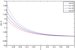
• Figure 1. Simulation of Example 1 with (a) $ \gamma = 0.0001 $, (b) $ \gamma = 0.001 $, and (c) $ \gamma = 0.1 $ for $ h = 0.1 $ and $ \Delta t = 0.001 $ at various $ t $
• Figure 2. 3D plots of $ u(x, t) $ for Example 1 with (a) $ \gamma = 0.0001 $, (b) $ \gamma = 0.001 $, and (c) $ \gamma = 0.1 $ for $ h = 0.1 $ and $ \Delta t = 0.001 $ at $ t = 0.2 $
• Figure 3. Plots for Example 2 with $ \gamma = 0.0001 $, $ h = 0.1 $, and $ \Delta t = 0.001 $ at different $ t $
• Figure 4. 3D plots of $ u(x, t) $ for Example 2 with $ \gamma = 0.0001 $ for $ h = 0.025 $, and $ \Delta t = 0.0001 $, where $ t\in[0.25, 5] $
• Figure 5. Plots for Example 3 with $ \gamma = 0.0001 $, $ h = 0.1 $, and $ \Delta t = 0.001 $ at different $ t $
• Figure 6. 3D plots of $ u(x, t) $ for Example 3 with $ \gamma = 0.0001 $ for $ h = 0.025 $, and $ \Delta t = 0.0001 $, where $ t\in[0.25, 5] $
• Figure 7. A comparison of the exact and numerical values of $ u(x, t) $ for Example 4 with $ \gamma = 1 $, $ h = 0.025 $, and $ \Delta t = 0.001 $ for $ t $ = 0.1, 0.3, 0.5, 0.7
• Figure 8. 3D plots of exact and numerical $ u(x, t) $ together with abs. norms for $ \gamma = 1 $ and $ \Delta t = 0.0005 $ with (a) $ h = 0.05 $ and $ t \in[0, 0.02] $, (b) $ h = 0.025 $ and $ t \in[0, 1] $ for Example 4